Grokking

 

LLM context is not optional

On numerous occasions, I have heard people say that GPT answers are generic, shallow, or otherwise insufficient.

I object to this opinion.

Not because the models are flawless, but because the criticism often misidentifies the problem's source.

Modern large language models represent a compressed statistical summary of an enormous portion of what has been publicly written.

They do not store documents. They encode patterns, structures, distinctions, and relationships across domains at a scale no individual human can internalize.

From the model’s perspective, there are only two things to work with.

One is the representation space shaped during training, which might be called learned meaning proximity in representation space.

The other is the context provided at inference time, the text we place in front of the model and ask it to continue.

The learned representation is undeniably powerful.

I have seen this directly when the model explained subtle distinctions in eighteenth-century Japanese poetry, including how classical grammar and social context are distorted in many modern translations.

That kind of response is not generic. It reflects the deep structure of the training data.

Where things often fail is the other half of the equation.

The context we provide as users is frequently vague, underspecified, or internally inconsistent.

We ask broad questions.

We mix goals.

We omit constraints.

We rely on unstated assumptions.

Then we blame the model for producing broad answers.

From the model’s perspective, a weak prompt defines a broad, blurry region of the meaning space.

When attention has nothing precise to lock onto, the output naturally gravitates toward statistically common, default responses, intellectually equivalent to the bad prompt that produced them.

This is not a flaw unique to LLMs. The same dynamic exists in human conversation.

Precise questions invite precise answers. Poorly-formed questions invite platitudes.

Seen this way, prompting is not a cosmetic skill.

It is the act of placing the model in the right neighborhood of meaning space.

Good context allows latent structure to surface.


In practice, when approaching a complex or scientific question, this means preparing a laser-focused conversational context.

That context may include notes that frame the question, references to recent innovations such as papers, articles, or news, and clearly stated constraints.


Very often, for fifteen or more minutes, I ask GPT to pose clarifying questions one at a time.

Only when I am confident it understands the problem precisely do I proceed and ask GPT to write a prompt for itself that summarizes the problem's mental framework as it understands it.


Only then do I have a real chance of receiving not a generic answer, but a concept or idea that has never been explicitly written down, yet emerges naturally as an intersection of existing concepts, algorithms, or solutions.

In other words, something genuinely novel.


It is well known that after an important speech or a major publication, multiple scientists often independently arrive at the same invention nearly simultaneously.

This is what it means to share the essential context.

Coqui

In my study of Deep Neural Networks (DNN), I wanted to explore text-to-speech (TTS).

One problem I wanted to solve is that my blog posts mix English and Japanese.

After exploring various TTS options, I switched from monolingual Japanese models to Coqui’s XTTS, a multilingual system that can speak English and Japanese in the same voice. The difference was immediate. Kokoro sounded OK for pure Japanese, but it forced English into Japanese phonetics. XTTS, on the other hand, handled mixed-sentence structures smoothly and maintained a consistent female voice across both languages.

I am happy to meet you、よろしくお願いします。Today we can study together、一緒に勉強しましょう。

With a few lines of code and a reference audio clip, XTTS generated natural-sounding speech for an entire paragraph, blending English greetings, simple Japanese phrases, and everyday expressions. Both languages were pronounced correctly, with tone and pacing that felt unified. Importantly, the model applied the same cloned voice to every line, exactly what I need for a bilingual macOS avatar.

The output quality is now good enough to move forward. The next step will be fine-tuning the model on a larger dataset of my own recordings, integrating the TTS pipeline into a SwiftUI interface, and eventually building a complete English-Japanese teaching assistant that speaks in a clear, friendly voice. An audiobook generator could be possible. For now, hearing mixed-language speech flow naturally from my own custom voice model feels like a small but meaningful success.

Drones

 

Principles

 I have been exploring a different way to think about physics in simulations. Instead of using object-oriented structures where each physical entity carries its own full behavior, I want to build a library of pure “first-principles forces.” Each force is its own small module, ideally a compact neural network, and each module acts like a tiny brain center that reads object properties and produces its own contribution to the world.

Objects in this system are nothing more than numeric data points. A water droplet, a dust particle, a photon, or a molecule is just a bundle of values such as position, velocity, mass, charge, temperature, or phase. No object contains its own methods. All behavior comes from the outside, from many small force networks evaluating the state at each step.

The simulation loop becomes simple. It holds a list of objects and a list of forces. Each force module looks at the current state and writes an influence, such as a force vector, a heat change, or a probability of phase transition. After all influences are collected, the system updates every object. The world is the sum of these small brains acting together.

This idea becomes especially attractive when dealing with very large numbers of tiny objects, such as water molecules nucleating into a droplet or photons passing through a medium. Classical physics code becomes messy when hundreds of thousands of items interact. A neural approach, where each phenomenon is a learned transformation, scales more naturally and can approximate complex interactions without hand-written formulas.

The long-term vision is a library of first-principles modules: inertia, drag, friction, buoyancy, pairwise gravity, electrostatic influence, thermal conduction, phase changes, and so on. Each module would be replaceable: analytic formulas when known, neural networks when unknown or too expensive to compute directly. This creates a flexible framework where simple rules, traditional physics, and learned behavior coexist.

For now this remains a conceptual sketch, but it suggests a path toward simulations that are more modular, scalable, and expressive. I can return to this idea later and explore how to structure the object schemas, how to train the small neural force networks, and how to combine them into a stable and useful physics engine.

Affordance is Play

Affordance as a Function of Intent and Action?

As a person passionate about Behavioral Sciences, I found myself unable to shake the impression that the paper “A Theory of Affordances in Reinforcement Learning” somewhat artificially imposes a mathematical frame on the idea. The authors, following Gibson in 1977, define “affordance” as a relationship between intent and action success within a Markov Decision Process (MDP). 

In their formulation, an affordance is something that fulfills an intended goal with a certain probability. 

The paper remains valid but inspires us to think more deeply about the meaning of affordance, especially in the context of Machine Learning.

Markov Decision Process (MDP) is a loop:

1. You (or agent) in some situation (personal and world state).
2. You (or agent) choose an action.
3. The world reacts (new state + reward).
4. Wash and repeat.

MDP fits neatly into the machinery of reinforcement learning, where an agent seeks to maximize rewards by executing optimal actions.

Gibson (1977) defined affordances as different possibilities of action that the environment affords to an agent.

I do not have an issue with Gibson's ecological definition. 

Affordance is Play

To me, affordance has less to do with intent and everything to do with play.

In the real world, we discover affordances not by planning but by playing with possibilities. 

A child learns what can be done by climbing, falling, touching, and testing the boundaries of safety. The best moments of childhood play are those when we barely escaped unscathed; when the heart raced, when something almost went wrong, but didn’t. That boundary between freedom and danger is where learning is deepest.

Affordance, in this sense, is not about achieving an outcome. It is about staying alive while experimenting with the world. 

It defines the space within which we can change the game's parameters without getting hurt. 

In reinforcement learning (RL) terms, it is the manifold of safe exploration, or the zone where feedback is rich but failure is not fatal.

source: Atlantic

 

Simulation and Safe Play

This form of learning is ancient. We simulate dangerous situations in imagination, running them over and over in the mind’s eye. Or we externalize them through ritualized, controlled play, just like in karate kata, where potentially lethal movements are practiced in a form that is safe and repeatable. Then there is karate kumite, or sparring, where we step closer to real risk but still within agreed limits. Both are forms of play. Both train us to recognize the edges of danger without crossing them.

It is the Most Serious Matter

Play, then, is not the opposite of seriousness; it is the method by which organisms map the terrain of survival. Through play, we learn about the world’s resistance and our own capabilities. The outcome of play is not a single intent achieved, but a widening of understanding; an embodied sense of what is possible.

The Definition

If I were to define affordance, I would not say it is “the subset of state–action pairs that fulfill intent.” I would say:

Affordance is the set of game parameters within which an agent can safely play and explore the outcomes that bring meaningful experiences.

It is the field of viable transformation, the space where curiosity meets consequence and both survive the encounter.

Mathematics

For those people who do not consider writing worth reading unless it contains at least 20% of LaTeX.

Let’s assume hazard H is a function that indicates how risky it is to take a particular action a in a given state s.

$$ H(s,a) \le h_{max} $$

If the hazard is below some acceptable threshold \( h_{max} \), then this action is considered safe enough to play with.
 In everyday terms: “Don’t jump higher than you can land safely.”

Now we introduce a second measure, feedback richness F. It describes how much change or learning happens when you take an action a. We can compute it by looking at the expected difference between the current state s and the next state s' after performing action a.

$$ F(s,a) = \mathrm{E}_{s' \sim P(\cdot \mid s,a)} \left[ D(s,s') \right] $$

where:

Symbol	Meaning
\( s \)	The current state of the agent.
\( a \)	The action taken in that state.
\( s' \)	Read “s-prime” — the next state that results after performing the action.
\( P(s' \mid s,a) \)	The transition probability: how likely it is to reach each possible next state \( s' \) when taking action \( a \) in state \( s \).
\( D(s,s') \)	A difference function measuring how much the world or the agent’s perception changes between \( s \) and \( s' \); it could represent distance, novelty, or information gain.
\( \mathbb{E}_{s' \sim P(s' \mid s,a)}[\cdot] \)	The expected value — the average of that difference over all possible next states following from \( s,a \).

The formula asks: “On average, how different is the world after I act?”
If nothing changes (like bouncing on a log that won’t move), feedback is low. If something new happens (the world reacts in an interesting way), feedback is high.
So \( F \) measures how informative or “fun” the action is: how much it teaches the agent about the world.

The affordance of play is the set of all state–action pairs that are both safe and interesting:

$$ A_{play} = \{ (s,a) \in S \times A \mid H(s,a) \le h_{max},\ F(s,a) \ge f_{min} \} $$

In plain language: An action is “playable” if it won’t hurt you and it’s worth doing because you might learn something new. It defines the zone of viable exploration; the sweet spot between boredom and danger.

Next, we define the play policy: the way an agent chooses its actions to keep playing safely and learning effectively.

$$ \pi_{play}^{*} = \arg\max_{\pi} E\!\left[ \sum_{t=0}^{T} \gamma^{t} F(s_t,a_t) \right] \quad \text{s.t.} \quad H(s_t,a_t) \le h_{max},\ \forall t $$

where:

Symbol	Meaning
\( \pi \)	A policy — a rule or function that tells the agent which action to take in each state.
\( \pi_{\text{play}}^{*} \)	The best (optimal) play policy that satisfies the safety rule.
\( \arg\max_{\pi} \)	Find the policy that gives the maximum possible value.
\( \mathbb{E}[\cdot] \)	The expected value, i.e., the average over all possible outcomes.
\( \sum_{t=0}^{T} \)	A sum over time steps from the beginning (\(t=0\)) until some horizon \(T\).
\( \gamma^{t} \)	A discount factor (0 < \( \gamma \) < 1) that slightly reduces the importance of far-future experiences; it models our natural tendency to value the present more than the distant future.
\( F(s_t,a_t) \)	Feedback richness — how much the agent learns from taking action \(a_t\) in state \(s_t\).
\( H(s_t,a_t) \)	Hazard — the expected risk or potential harm of taking that action.
\( h_{\max} \)	The maximum acceptable hazard, the safety limit.
\( H(s_t,a_t) \le h_{\max} \)	The safety constraint: every action must remain below the danger threshold.

This formula means the agent tries to maximize total feedback over time (it wants the richest learning experience possible) while keeping every action within the safety boundary. 

In other words: “Explore as much as you can without getting hurt.”

The factor \( \gamma \) (gamma) discounts future feedback slightly, just as we naturally prefer immediate experiences to distant ones.

For comparison, the classical reinforcement learning policy focuses purely on reward:

$$ \pi^{*} = \arg\max_{\pi} E\!\left[ \sum_{t=0}^{\infty} \gamma^{t} r(s_t,a_t) \right] $$

Traditional Reinforcement Learning (RL) agents chase rewards \( r \). 

A playful agent instead chases understanding \( F \), which signals curiosity, while respecting a safety boundary \( H \). 

 It is not optimizing for success but for continued participation.

Application for Machine Learning

In practical machine learning, this perspective turns into a guide for building better agents. Instead of rewarding an agent only when it achieves a fixed goal, we can encourage it to discover where it can play safely. The agent learns the boundaries of its world and the regions that respond richly to its actions, rather than blindly optimizing for external rewards.

In reinforcement learning terms, the agent can maintain two learned functions: a hazard model \( H(s,a) \) estimating the probability of failure or damage, and a feedback model \( F(s,a) \) estimating the expected amount of new information or improvement gained from an action. By combining them, the agent can create its own playground of exploration \( A_{play} \) and focus on safe and informative actions.

Such agents do not merely chase rewards; they evolve through curiosity. 

They learn the structure of their environment by interacting with it, not just memorizing outcomes. This approach aligns machine learning more closely with how humans and animals learn: through playful experimentation, through testing what can be changed without harm. It is learning as a continuous dance with uncertainty; an art of exploring the edge of safety where discovery happens.

References

• “A Theory of Affordances in Reinforcement Learning”, Khimya Khetarpal et al. https://arxiv.org/pdf/2006.15085
  

Recurrent Neural Network (RNN) cell in PyTorch

This minimal PyTorch example implements a custom recurrent neural network (RNN) cell from first principles, showing how sequence memory emerges through feedback.

The cell maintains a hidden state vector h, which evolves over time using the current input x and the previous hidden state through the nonlinear update h = tanh(Wₕₕh + Wₓₕx). The output y = Wₕy h is then computed as a simple linear projection of the hidden state.

Unlike PyTorch’s built-in nn.RNN, this implementation makes every matrix and operation explicit, clearly illustrating how temporal dependencies are learned through recursive state updates rather than static input-output mappings.

code: https://github.com/UkiDLucas/DNN-book

import torch
import torch.nn as nn

# pick device (use "mps" on Apple Silicon;
# macOS Metal hardware acceleration
device = torch.device("mps" if torch.backends.mps.is_available() else "cpu")

class MyRNNCell(nn.Module):

# rnn_units: number of hidden neurons
def __init__(self, rnn_units, input_dim, output_dim):

super().__init__()

# weight matrices, * 0.01 scales the random weight initialization to small values

self.W_xh = nn.Parameter(torch.randn(rnn_units, input_dim) * 0.01)

self.W_hh = nn.Parameter(torch.randn(rnn_units, rnn_units) * 0.01)

self.W_hy = nn.Parameter(torch.randn(output_dim, rnn_units) * 0.01)

# hidden state h initialized to zeros

self.register_buffer("h", torch.zeros(rnn_units, 1))

def forward(self, x):

# x is shape [input_dim, 1]

self.h = torch.tanh(self.W_hh @ self.h + self.W_xh @ x)

y = self.W_hy @ self.h

return y, self.h

# minimal usage example

if __name__ == "__main__":

rnn = MyRNNCell(rnn_units=16, input_dim=8, output_dim=4).to(device)

x_t = torch.randn(8, 1, device=device) # input vector at time t

y_t, h_t = rnn(x_t)

print(y_t.shape, h_t.shape) # torch.Size([4, 1]) torch.Size([16, 1])

A practical use of this minimal RNN cell is to predict or generate sequential data, where each step depends on the previous one.

For example:

• Time series forecasting: Feed in one value at a time (like daily temperatures or stock prices) and train it to predict the next value.

• Character-level text generation: Convert characters to one-hot vectors, feed them sequentially, and let the RNN learn to predict the next character.

• Signal smoothing or sensor prediction: Use it to process sequential readings (like a boat’s wind and wave sensors) to predict future conditions.

Even though it’s a tiny model, it demonstrates the whole idea: maintaining internal memory (h) to connect past inputs with future outputs.

Various RNN configurations:

• single input >  RNN cell > single result for binary classification
• many inputs > many RNN cells > single output: sentiment classification
• single input > many RNN cells > many outputs: text generation, image captions
• many inputs > many RNN cells > many outputs: translation, music generation

Think of an RNN as a storyteller that remembers what has already been said while deciding what comes next. Each RNN cell is like one frame in a film reel—receiving new input, updating its memory, and passing that memory forward. When you connect many cells in series, the network forms a chain of thought through time: it doesn’t see the whole story at once but recalls what just happened. In a simple one-to-one setup, it’s like hearing a single word and deciding “yes” or “no.” With many inputs feeding into a single output, it listens to a whole sentence before forming an opinion, such as judging sentiment. With one input producing many outputs, it’s as if the RNN takes one idea and tells a whole story, step by step. And when many inputs produce many outputs, it becomes a fluent translator or composer—listening, remembering, and responding continuously.

References:

• https://github.com/UkiDLucas/DNN-book?
• https://www.youtube.com/watch?v=GvezxUdLrEk&list=PLtBw6njQRU-rwp5__7C0oIVt26ZgjG9NI

Best Neural Network framework to run on macOS M1.

Choosing the best Neural Network framework to run on my macOS M1 64 GB RAM workstation.

Neural network frameworks on macOS M1 with native acceleration

Framework	Programming language	M1 acceleration rating
PyTorch (MPS backend)	Python, C++	9/10
TensorFlow + tensorflow-metal	Python, C++	8/10
Core ML (inference)	Swift, Python bridge	10/10
ONNX Runtime (Core ML/Metal delegate)	C++, Python API	7/10
JAX (Metal backend)	Python	6/10
MXNet	Python, C++	3/10
CNTK	Python, C++	3/10
Theano	Python	3/10

Free MIT.edu OpenWare Courses (OWC)

MIT.edu OCW

Designed for 6–7 months of structured, portfolio-driven study (10–12 hrs/week)

OCW study sequence for AI/ML and robotics foundations

Order	Course	Theme	Duration (weeks)	Application tie-in
0	6.S191 – Introduction to Deep Learning	Modern deep-learning foundations (CNNs, RNNs, Transformers)	4	TensorFlow/PyTorch hands-on intro; vision, NLP, biology
1	6.042J – Mathematics for Computer Science	Discrete math and graphs	3–4	SLAM topologies, graph optimization
2	6.041SC – Probabilistic Systems Analysis and Applied Probability	Probability and systems	4–5	Sensor fusion, Bayesian estimation, uncertainty modeling
3	6.036 – Introduction to Machine Learning	Core machine learning	4–6	Classification, regression, regularization
4	6.801 – Machine Vision	Vision and perception	4–5	Mapping, feature detection, optical flow, 3D reconstruction
5	6.4210 – Robotic Manipulation	Robotics and control	5–6	Motion planning, control loops, state estimation
6	9.01 – Introduction to Neuroscience	Biological neural systems	3–4	Sensory pathways, motor control, neural coding
7	9.13 – The Human Brain	Cognitive neuroscience	3	Perception, learning, memory architecture
8	9.40 – Introduction to Neural Computation	Computational neuroscience	4–5	Modeling neurons and learning rules
9	9.66J – Computational Cognitive Science	Cognitive modeling	4–5	Probabilistic reasoning, human-like perception
10	9.85 – Infant and Adult Cognition	Learning and development	2–3	Developmental and reinforcement models

Classification - Machine Learning with Python - IBM AI Engineering certificate program on Coursera

NOTE: This is a continuation of the: "IBM AI Engineering certificate program on Coursera - Machine Learning with Python"

https://uki.blogspot.com/2022/09/ibmaiengineering.html

Please note that the Mathematic formulas (LaTex script) DO NOT show on the MOBILE phone, to read this post please use the desktop Chrome browser.

All images are copyrighted by IBM Developer Skills Network.

Table of Contents

• Introduction to Classification
• k-Nearest Neighbors
• 
  

 Introduction to Classification

https://www.coursera.org/learn/machine-learning-with-python/lecture/95g22/introduction-to-classification

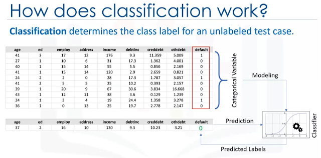
What is classification?

• Classification is a supervised machine learning approach
• Categorizing some unknown items into a discrete set of categories or "classes".
• Relationship between "feature" variables and the target attribute which is a categorical variable.

What is multi-class classification?

Multi-class classification can predict the target attribute (a field) with multiple discrete values to choose from.

What are examples of Multi-class classification use cases?

• category to which the person belongs
• churn detection: person switching brand loyalty
• detect if a person responds to a particular advertising campaign

What are the types of classification algorithms?

• Decision Trees (ID3, C4.5, C5.0)
• Naïve Bayes,
• Linear Discriminant Analysis
• k-Nearest Neighbor
• Logistic Regression
• Neural Networks (DNN)
• Support Vector Machines (SVM)

k-Nearest Neighbors (kNN)

https://www.coursera.org/learn/machine-learning-with-python/lecture/s0q1d/k-nearest-neighbours

K-Nearest Neighbors is a supervised learning algorithm. Where the data is 'trained' with data points corresponding to their classification. To predict the class of a given data point, it takes into account the classes of the 'K' nearest data points and chooses the class to which the majority of the 'K' nearest data points belong as the predicted class.

• The kNN algorithm is a classification algorithm
• The kNN algorithm classifies classes on their similarity to other classes 
• The kNN can work with Minkowski/Eucleadian distance, but it does not have to.
• The large, or the small, size of k in kNN does guarantee a good model, rather the k value needs to be found empirically.
• kNN can be used to compute a continuous value, for example, the price of a home

How to determine which class?

Find several nearest neighbors in the data (e.g. age, income, etc.) and determine (vote) to which class they should belong.

This can be done using Euclidean Distance [reference 1].

How does the k-Nearest Neighbor work?

• pick a value for K
• calculate the distance of the unknown case from all cases
• select the k-observations in the training data that are "nearest" to the unknown data point
• predict the response of the unknown data point the most popular response value from the K-nearest neighbors.

How to select the K-value?

• too small of the k sample may capture the "noise" in the data (an outlier)
• a low value of k makes for a very complex model which may result in overfitting of the model
• too large of the k can make the model overgeneralized
• reserve part of your data to test the distribution of accuracy of the model for various k= 1 to n

How to calculate the distance between k-neighbors?

• We can use the Minkowski distance (aka Euclidean distance)
• normalize the unites

$$
Minkowski \ distance (x_1, x_2) =
\sqrt{
  \sum_{i=0}^{n}
  \left(
    x_{1i} - x_{2i}
  \right)^2 
} 
$$

Example (not normalized):

• person 1
• age 34
• income 190
• education 3
• person 2
• age 30
• income 200
• education 8

$$
Minkowski \ distance (x_1, x_2) =
\sqrt{
  \sum_{i=0}^{n}
  \left(
    x_{1i} - x_{2i}
  \right)^2 
} 
$$

$$ = \sqrt{  \left( 34 - 30 \right)^2 + \left( 190 - 200 \right)^2 + \left( 3 - 8 \right)^2 }  \\ = 11.87 $$

Evaluation Metrics in Classification

https://www.coursera.org/learn/machine-learning-with-python/lecture/5iCQt/evaluation-metrics-in-classification

Harmonic Mean [see references 2, 3 ]

$$ harmonic \ mean  = \frac{2*A*B}{A+B} $$

Classification Accuracy

compare the historical actual data $ y $ vs predicted values $ \hat{y} $

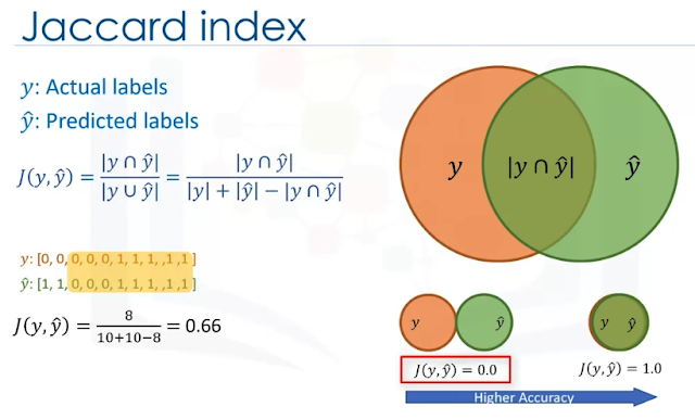
• Jaccard index (similarity coefficient, intersection-over-union)

• F1 score (Confusion matrix)
• TP = True Positives
• FN = False Negatives
• FP = False Positives
• TN = True Negatives
• precision = TP / (TP + FP)
• use when identifying positives is a priority
• example: classify butterfly species
• recall  = TP / (TP + FN) 
• use when false negatives are a problem
• example: identify non-existing obstacles at highway speed
• F1 score is a harmonic mean of the precision and recall scores
• F1 score = $ \frac{2 * precision * recall}{precision + recall} $ 
• Finally, we can average multiple F1 score results

Logarithmic (Log) Loss

• Sometimes the output is the probability of the class label
• continuous values between 0 to 1 (or 0 to 100%, or NO to YES)
• Log Loss measures the performance of the classifier where the output is a probability

$$ error = y \cdot log(\hat{y}) + ( 1 -y ) \cdot \log(1 - \hat{y}) $$

Where:

• $ \hat{y} $ is a predicted result
• y is the actual observed result

Then, we can calculate the Log Loss as an average across all observations (rows n):

$$ LogLoss = - \frac{1}{n} \sum_{i=1}^{n} ( error_i ) $$

The classifier with the lower Log Loss has better performance.

Lab: kNN

https://www.coursera.org/learn/machine-learning-with-python/ungradedLti/pUIUL/lab-knn

References

1. https://en.wikipedia.org/wiki/Euclidean_distance
2. https://en.wikipedia.org/wiki/Harmonic_mean
3. https://en.wikibooks.org/wiki/Statistics/Summary/Averages/Harmonic_Mean
4. https://www.coursera.org/learn/machine-learning-with-python/lecture/5iCQt/evaluation-metrics-in-classification
5. lab kNN: https://www.coursera.org/learn/machine-learning-with-python/ungradedLti/pUIUL/lab-knn

Image Perception on Inexpensive Embedded Hardware

When people hear “machine learning,” they often imagine large models running on powerful GPUs in data centers. That picture breaks down quickly once we move to edge devices. Cameras, LiDAR sensors, vehicles, and especially drones operate under tight constraints: limited power and thermal budget, strict latency requirements, and often no access to cloud resources. In these environments, the question is not how powerful a model can be, but how efficiently practical computation can be performed.

Image matching in perception is a good example. We start with raw red, green, and blue (RGB) values for every pixel. Even a modest image contains millions of such values. Processing all of them directly is neither necessary nor efficient. Instead, perception systems select small regions of interest and reduce them to compact numeric representations that can be compared across images. These representations allow a system to recognize the same physical point despite camera motion, rotation, or slight changes in lighting.

A common approach is to extract a small image patch (or kernel) at a time. For example, an 8×8 grayscale patch captures local structure without excessive data. The goal is not to preserve every pixel, but to capture enough information so that the patch can be reliably matched to a corresponding patch in another image. This step already reflects a core edge-computing idea: reduce data early, before it becomes expensive to move or process.

Traditionally, this reduction has been done with hand-designed feature descriptors. These methods rely on fixed mathematical operations, such as gradient comparisons or intensity differences, to produce a compact signature. While effective, they are rigid. Small neural networks provide an alternative that is still lightweight but more adaptable. Instead of hard-coding how pixel values should be combined, the network learns those combinations from data.

In this post, I start with a minimal deep neural network that performs this role. The deep neural network (DNN) operates on a small set of numeric inputs derived from an image patch and produces a short descriptor vector. The network is intentionally simple, consisting of two fully connected layers with a thresholding step between them. There is no recurrence, no attention, and no dynamic behavior. Every input produces an output in a fixed number of operations.

This simplicity is not a limitation. It is a design choice driven by edge constraints. A network of this size can be evaluated with predictable latency and minimal memory access. It can be quantized to fixed-point arithmetic without complex error behavior. Most importantly, it maps naturally onto hardware.

A Python implementation is a practical starting point because it allows the algorithm to be expressed clearly and tested quickly. However, Python is not the target execution environment. Running this computation on a CPU means executing many small arithmetic operations sequentially, with overhead that dominates the actual math. GPUs improve throughput, but at a cost in power and system complexity that is often unacceptable in embedded platforms.

On a system on a chip (SOC) like TI’s TDA4, this kind of workload can already be accelerated without a GPU. The device includes a C7x DSP paired with a Matrix Multiply Accelerator (MMA) designed specifically for dense linear algebra and neural network inference. Dense layers map naturally onto this hardware, while simple activation functions and distance calculations run efficiently on the DSP itself. This makes TDA4 a strong example of how edge processors are evolving toward integrated ML acceleration. At the same time, devices in this class typically fall in the $16 to $20 range in volume, which is entirely reasonable for automotive or industrial systems but still too expensive for many low-cost or highly specialized designs.

This cost boundary is one of the motivations for exploring FPGA and ASIC-style implementations, where a narrowly focused accelerator can deliver the required functionality at lower power and potentially lower unit cost.

On an FPGA or later on an ASIC, the computation becomes the structure of the circuit. Multiplications, additions, and comparisons happen in parallel, every clock cycle. Data flows through the network in a fixed pattern, producing one descriptor after another with deterministic timing. For workloads such as image matching, this approach aligns much better with edge requirements.

In the following blogs, I will expand on these ideas step by step.

What is Neural Network (NN)? by 3Blue1Brown

The video discusses:

• handwritten digit recognition example
• kernel size 28x28 pixel = 784 array
• activation layer 784 (1-dimensional) array 
• 2 hidden layers, each with 16 neurons (arbitrary choice)
• hidden layers correspond to macro and micro features within the digit
• 
  
  
  
  
• output layer 0..9, the largest value is the most likely selection of the NN
• He notes that the same principle can be applied to speech recognition.
• neuron parameters: knobs to adjust
• weights: connections between neurons
• activation function: normalizes the values between 0..1

https://www.youtube.com/watch?v=aircAruvnKk&list=PLZHQObOWTQDNU6R1_67000Dx_ZCJB-3pi&index=3